


In the previous post we waded theory-first into expected value (EV), and — acknowledging that having a +EV strategy doesn’t guarantee profit, the factors which impact the growth of our bankroll when we do have an edge. We came to the realisation that proving our strategies are +EV based on their historic results is an endeavour that rewards patience, volume, low odds, and relative indifference to any short-term results. But after considering parameters we could tweak, such as edge percentage, odds range, and total volume to improve this situation, there was one aspect which was conspicuously missing: Staking.
As one can imagine, we are not running into a unique problem by looking at this. In fact, since this problem touches anything where winnings compound and losses accumulate, basically all of the work has been done for us by clever people in the 1950s. Whilst it isn’t quite DNA or the polio vaccine, for us we’re looking at John Larry Kelly Jr.’s ‘Kelly Criterion’, which maximises the log-growth of the bankroll per-bet.
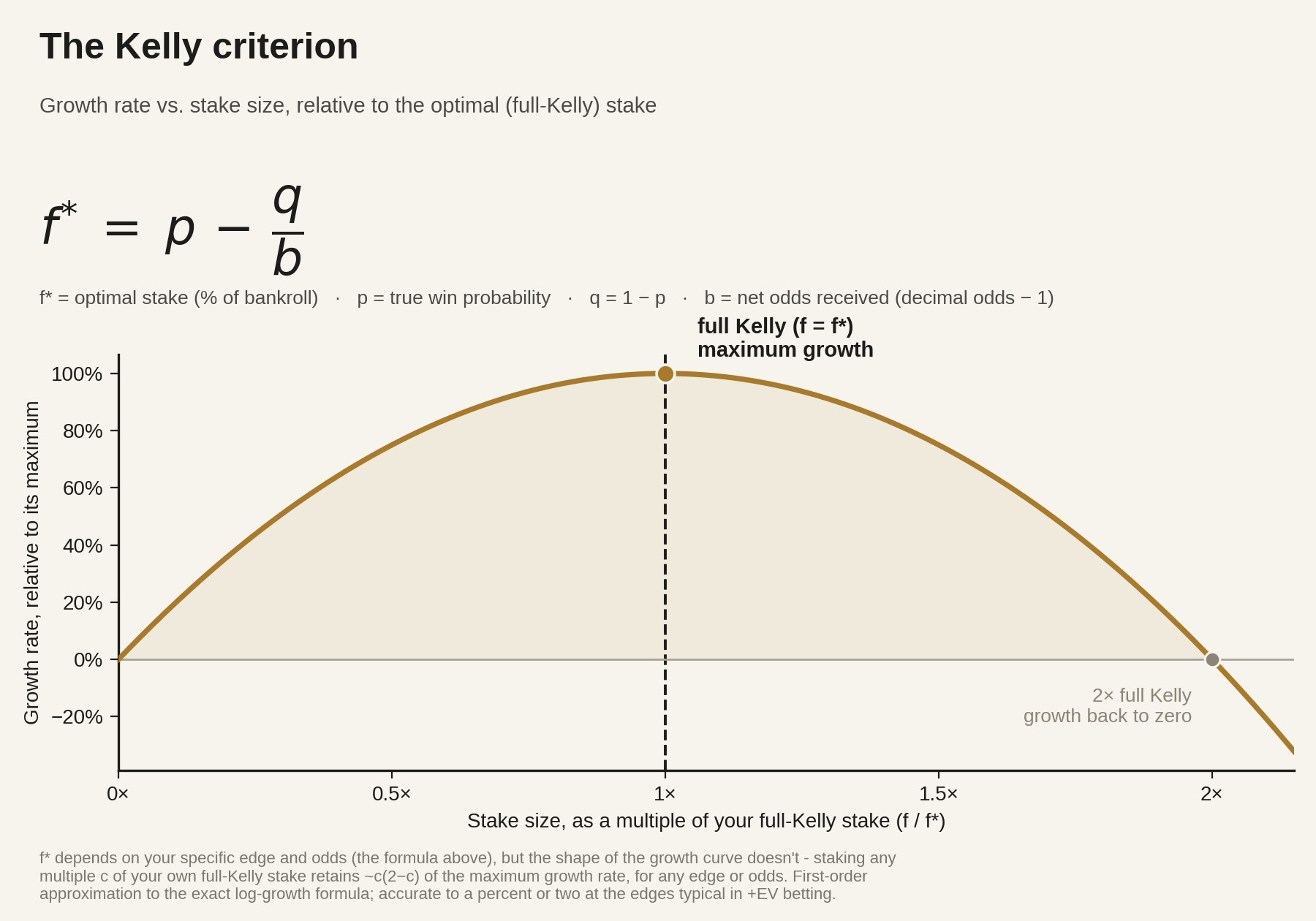
Intuitively, if we have an edge, we want to bet as big as possible, unless we’re betting so big that we’re in mathematically unsound levels of danger of our bankroll dropping to 0. And that is likely to depend on the size of our edge, and the likelihood of a winning payoff.
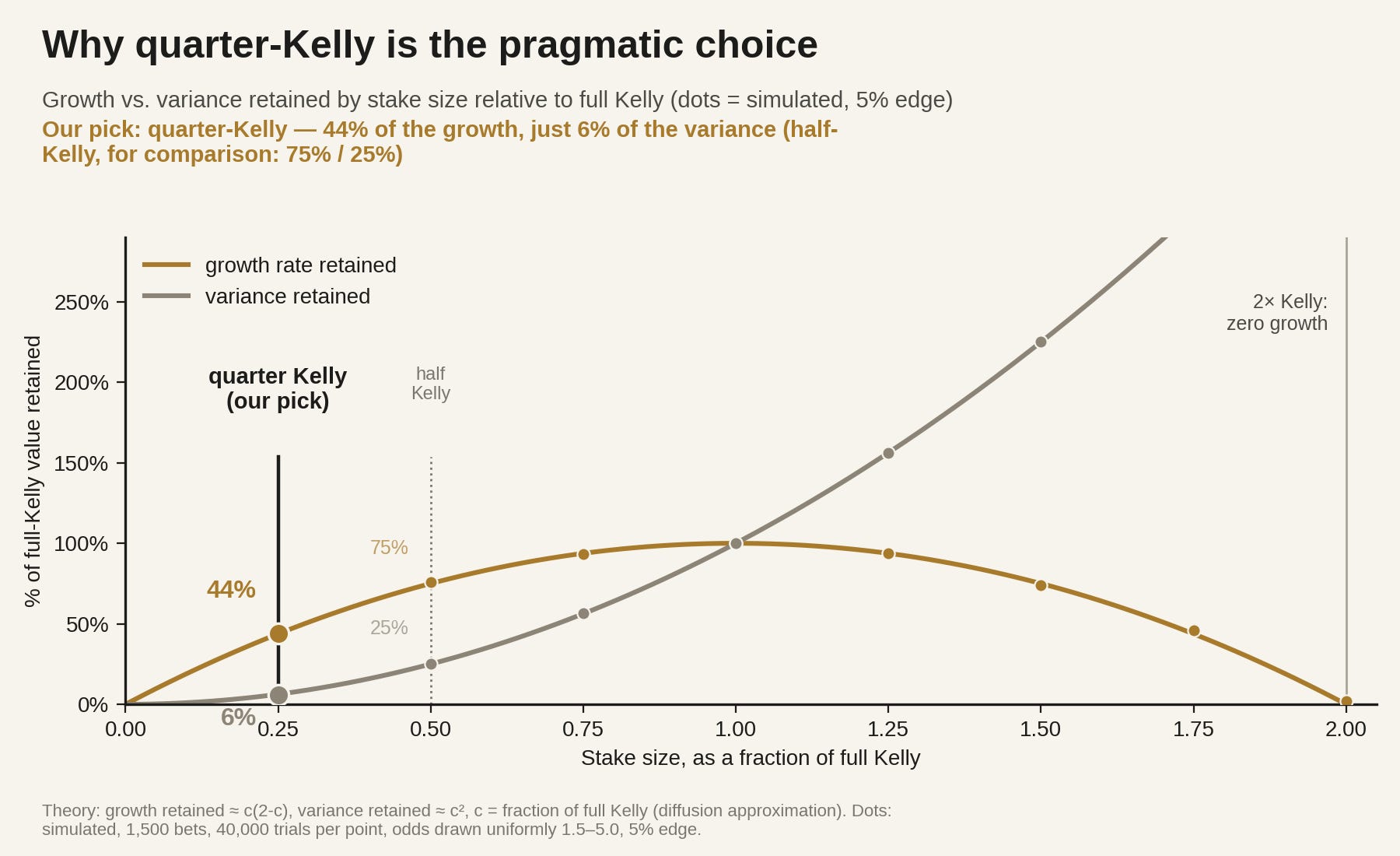
However, we do need to caveat our excitement slightly. Full-Kelly (betting the full fraction suggested) is brutally heavy on variance, sometimes requiring atomic-grade wagers of 20-40% of our bankroll depending on the probabilities involved. To retain the benefits of dynamic staking whilst minimising variance we typically pick a fractional Kelly regime, which significantly reduces the variance whilst preserving proportionally more bankroll growth. In past experiments I’ve used quarter-Kelly which has generally served me well, preserving 44% of the bankroll growth of full-Kelly, whilst subjecting our wallets and blood pressure to a much-reduced 6% of full-Kelly’s variance.
But, as nice as this has been so far, does it actually make a significant difference versus flat staking? In particular, if we’re going to implement this we at least want to be confident it will increase the growth of our bankroll. Let’s imagine we’ve found 1,000 bets, ranging from 2-8% in edge, and at odds 2.0 to 5.0. Unit staking or Kelly?
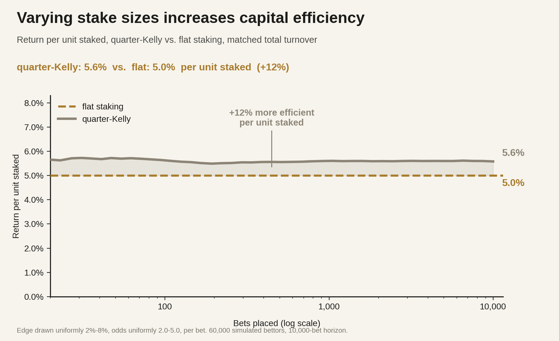
So in the figure above, we see that by varying our stake sizes with our estimate of the true edge, we generate an additional 0.6% ROI over the simulated runs. This is pretty significant; inevitably in the world we’re going to inhabit we’re going to have different projected edges and different odds, and a staking regime that ups our ROI by 0.6 percentage points is a very tidy outcome.
As with seemingly everything we cover, a word of caution is required. Whilst the above experiment enjoys the absolute privilege of knowing its exact edge, we almost certainly won’t in the strategies we’ll cover over the rest of this series. If a miscalibrated model starts putting more capital behind bets which have a lower true edge, far from enjoying a higher ROI we’ll instead suffer decreasing returns.
Speaking of knowing our true edge, the central thrust of Q1-03 was that this is actually really quite complicated. For good, liquid markets, we can use CLV. The statistical bar for proving our strategy is valid using CLV is much lower than drawing conclusions from our betting history. Our outcomes are no longer either winning or losing a bet, with all of the accompanying variance, but a comparison of the odds we’ve bet at versus the CLV, which is much more stable.
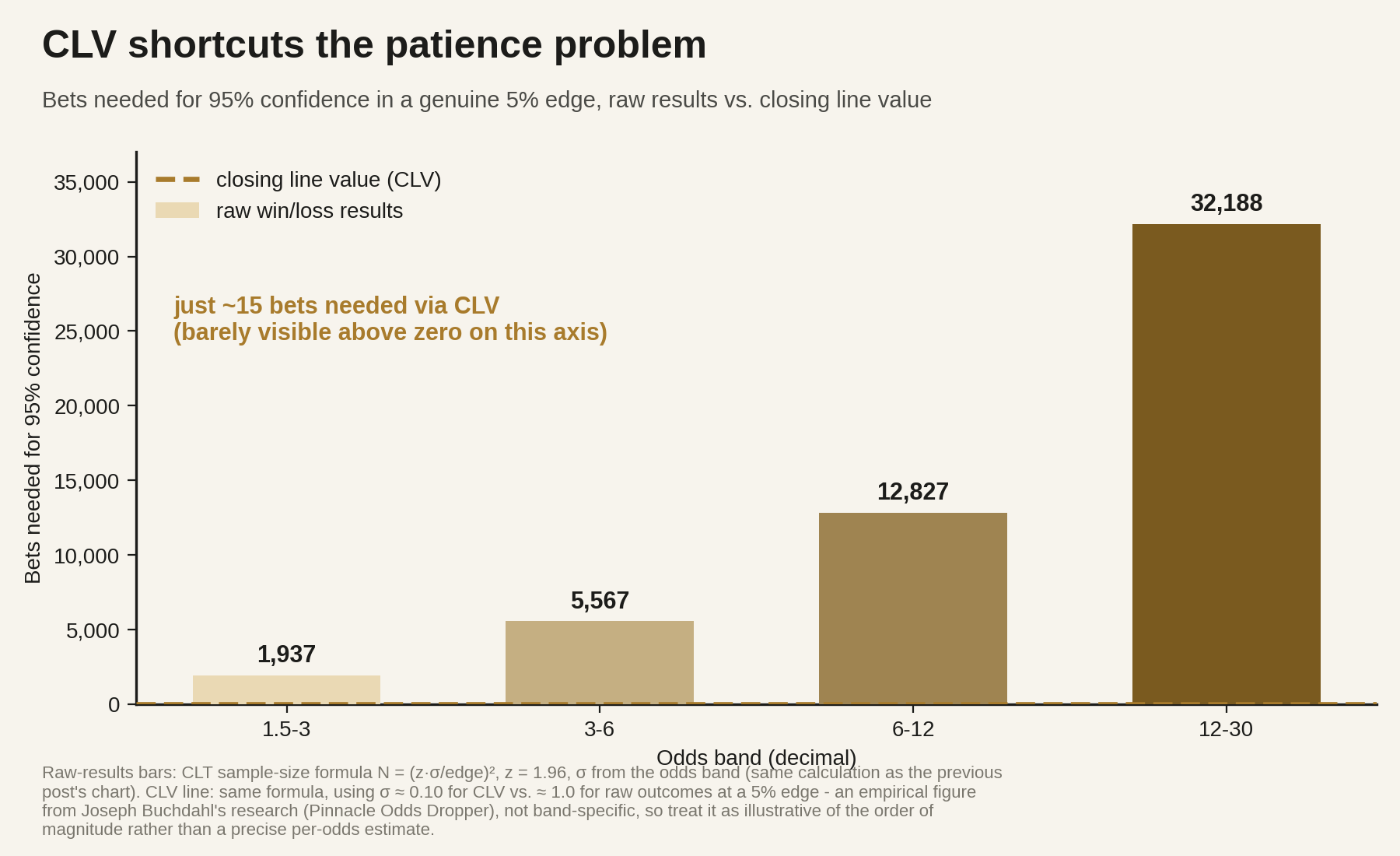
But if we want to go into more niche markets, CLV is less accurate for comparison. We need to look at our dataset and analyse it to identify whether there’s sufficient evidence to reject the null, and rather depressing hypothesis that we’ve not achieved anything meaningful edge-wise. This is simply a function of lower limits leading to less intensive price-discovery.
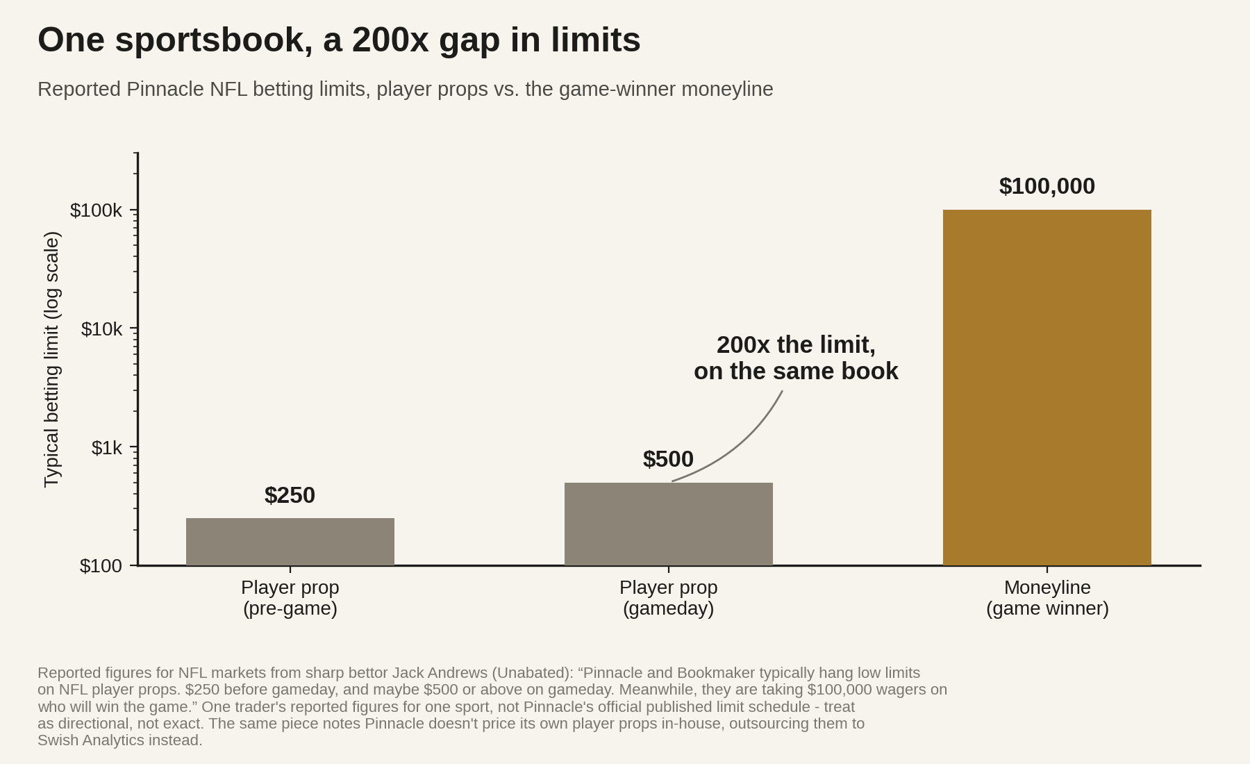
Source (exact figures aren’t watertight but there is a significant difference in limits for player props versus moneyline bets).
Does our newfound knowledge of staking regimes change the picture? Not in the strict sense. Adjusting our stakes up and down doesn’t change the underlying maths, which are entirely a function of betting outcomes. We can't manufacture evidence that an edge exists by deciding to risk more or less money on it. But in discussing staking we’ve opened up the dataset to be a better fit for reality — varying odds, varying edges. This can lead to alternative statistical methods that attempt to quantify whether our estimates of our edges is correct, such as log loss and brier score, meaning there is more out there to explore once we’re up and running some strategies.
But for now, where do we stand:
Staking regimes in dynamic edge environments actually matter and yield additional ROI over sequences of bets.
Quarter-Kelly is our regime of choice to preserve bankroll growth whilst minimising variance.
Proving our strategies are +EV is still painful unless we have strong CLV data.
Looking at alternative statistical methods can yield additional information about our betting performance.
Theory over, next post we’re going to finally delve back into The Research Desk and discuss a specific strategy I’ve been running over the past few weeks, which has yielded positive results. Looking forward to seeing you there.
The Alternative Desk
Still a going concern